Applying Specialized Conditional Formatting Using Data Bars : Conditional Formatting « Format Style « Microsoft Office Excel 2007 Tutorial

1. Microsoft Office Excel 2007 Tutorial
2. Format Style
3. Conditional Formatting

Select a cell or a range. 
           Click the Home tab. 
           Click the Conditional Formatting button. Point to Data Bars. 
           Click the colored data bar: Blue, Green, Red, Orange, Light Blue, or Purple.

To create a custom data bar, click More Rules

Specify the options. Then click OK.

Check the result.

3.10.Conditional Formatting
	3.10.1.	Conditional Formatting: Format Cell Contents Based on Comparison
	3.10.2.	Conditional Formatting: Format Cell Contents Based on Ranking and Average
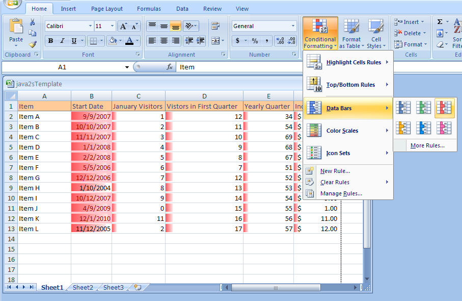
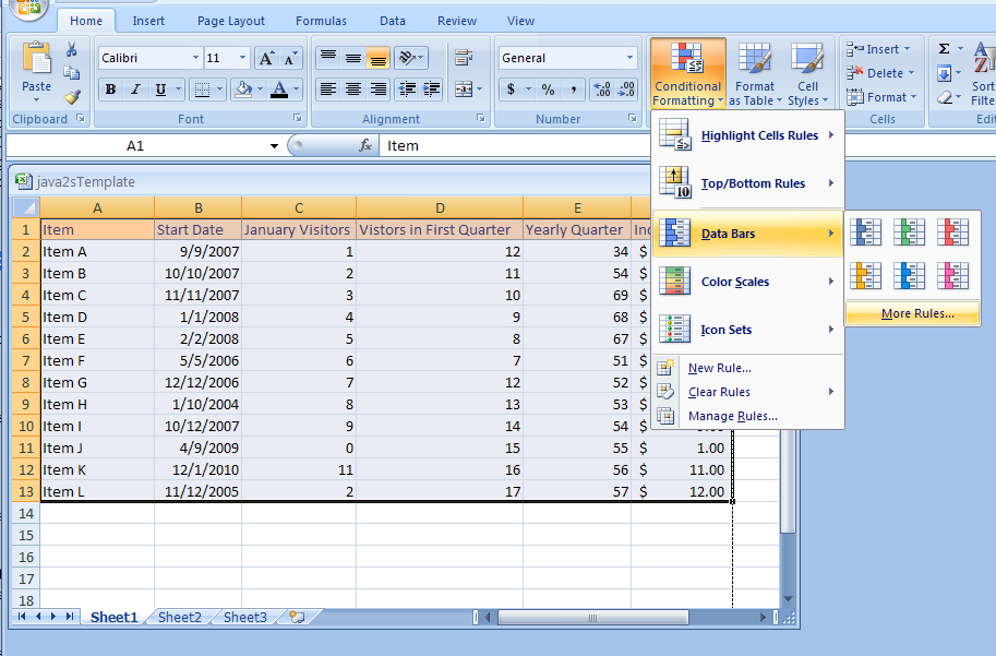
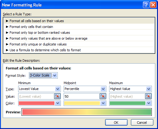
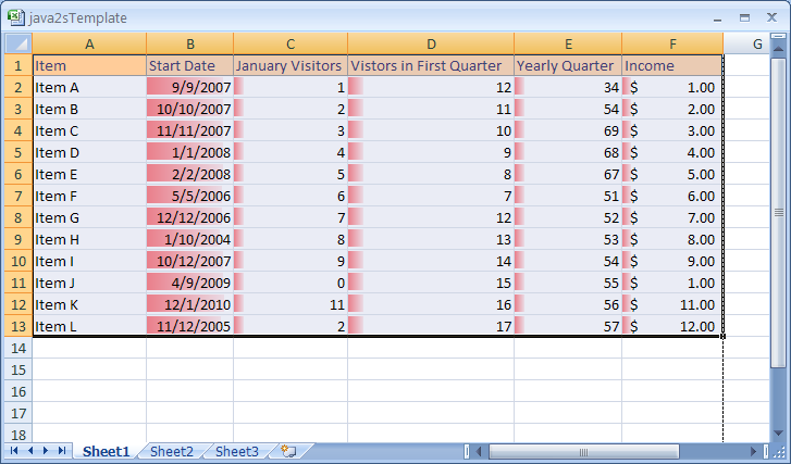
	3.10.3.	Applying Specialized Conditional Formatting Using Data Bars
	3.10.4.	Format Using Color Scales
	3.10.5.	Format Using Icon Sets
	3.10.6.	Create Conditional Formatting Rules
	3.10.7.	Clear Conditional Formatting Rules
	3.10.8.	Edit Conditional Formatting Rule Precedence