Conditional Formatting: Format Cell Contents Based on Ranking and Average : Conditional Formatting « Format Style « Microsoft Office Excel 2007 Tutorial

1. Microsoft Office Excel 2007 Tutorial
2. Format Style
3. Conditional Formatting

Select a cell or a range. 
           Click the Home tab. 
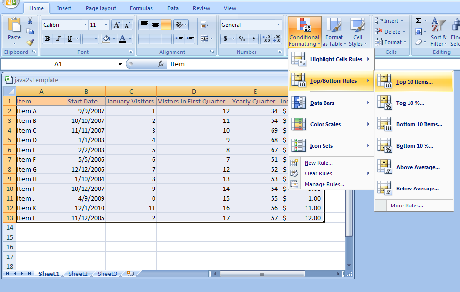
           Click the Conditional Formatting button. 
           Point to Top/Bottom Rules. 
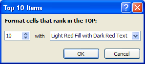
           Click the comparison rule: Top 10 Items, Top 10 %, Bottom 10 Items, Bottom 10 %, Above Average, Below Average

Specify the criteria. Click OK.

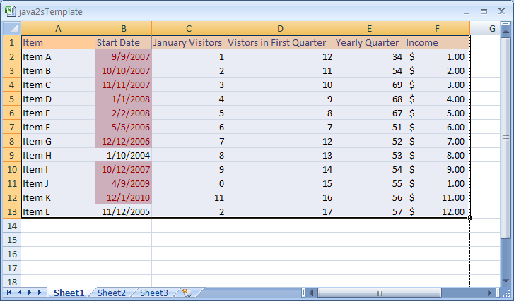
Check the result.

3.10.Conditional Formatting
	3.10.1.	Conditional Formatting: Format Cell Contents Based on Comparison
	3.10.2.	Conditional Formatting: Format Cell Contents Based on Ranking and Average
	3.10.3.	Applying Specialized Conditional Formatting Using Data Bars
	3.10.4.	Format Using Color Scales
	3.10.5.	Format Using Icon Sets
	3.10.6.	Create Conditional Formatting Rules
	3.10.7.	Clear Conditional Formatting Rules
	3.10.8.	Edit Conditional Formatting Rule Precedence